

The normal distribution was first described by Abraham Demoivre (1667-1754) as the limiting form of binomial model in 1733. Normal distribution was rediscovered by Gauss in 1809 and by Laplace in 1812. Both Gauss and Laplace were led to the distribution by their work on the theory of errors of observations arising in physical measuring processes, particularly in astronomy. Here I will show you some important properties of Normal distribution
1. The normal curve is “bell-shaped” and symmetrical in nature. The distribution of the frequencies on either side of the maximum ordinate of the curve is similar to each other.
2. The maximum ordinate of the normal curve is at \(X=m\). Hence the mean, median and mode of the normal distribution coincide.
3. It ranges between \($-\infty$\) to \($+\infty$\).

4. The value of the maximum ordinate is
5. The points where the curve change from convex to concave or vice versa is at
6. The first and third quartiles are equidistant from the median.
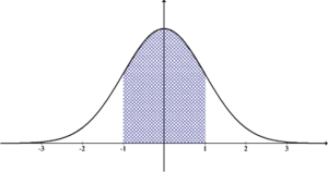
7. The area under the normal curve distribution is:
a.

b.

c.

8. When μ = 0 and σ = 1, then the normal distribution will be a standard normal curve. The probability function of standard normal curve is
Also read: How to check Multivariate normality using R?
The following table gives the area under the normal probability curve for some important value of Z.
|
Distance from the mean ordinate in Terms of ± σ |
Area under the curve |
|
Z = ± 0.6745 |
0.50 |
|
Z = ± 1.0 |
0.6826 |
|
Z = ± 1.96 |
0.95 |
|
Z = ± 2.00 |
0.9544 |
|
Z = ± 2.58 |
0.99 |
|
Z = ± 3.0 |
0.9973 |
9. All odd moments are equal to zero.
10. Skewness = 0 and Kurtosis = 3 in normal distribution.
Subscribe SAR Publisher and give your feedback, suggestions in the comment section.


